MCCE Mechanism
A MCCE simulation is a 4-step procedure:
- Step 1: __M__odify PDB (file formatting)
- Step 2: __C__onformer/Rotamer making
- Step 3: __C__alculate energy look-up table
- Step 4: __E__xtract microstates; Monte Carlo sampling of conformers at each pH or Eh
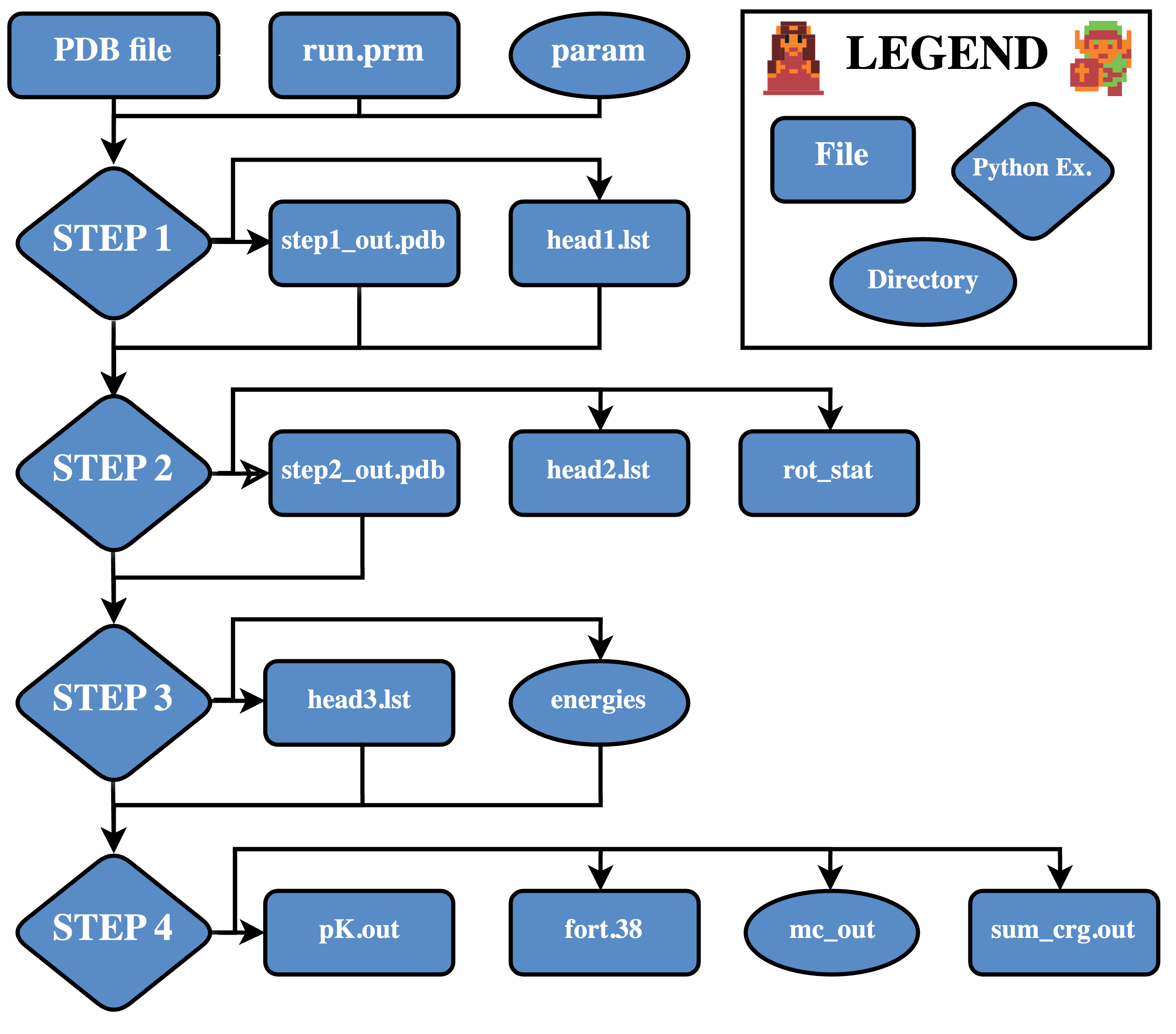
MCCE program can run any steps providing the prerequisite files exist in the working directory. Files required and written out by the program are illustrated in this chart. This file flow chart shows the summary of file dependencies:
Step 1: Modify PDB
Input Files
- PDB file – PDB format input file (must be in running directory)
Output Files
acc.res– Solvent accessibility of residuesacc.atm– Solvent accessibility of atomsnew.tpl(not always created) – Parameter file template of unrecognized cofactorshead1.lst(optionally used by Step 2) – Summary of rotamer making policy of residuesstep1_out.pdb(used by Step 2) – Step 1 output file in MCCE extended PDB format
Step 1 prepares an extended PDB file, suitable to be read into step 2. The input PDB file is in standard PDB format. It can have alternative side chain positions, but MCCE can’t process alternative backbone positions. Alternative side chains are treated as side chain conformers. When side chain atoms are missing, MCCE will complete the side chain atoms at the torsion minimum. In this step several things will happen:
With the instructions in the renaming rule file “name.txt”, residues and atoms will be renamed so that a cofactor can be split into several independent ionizable groups (for example, heme can be divided into heme and two propionates) and several groups can be combined as one (for example, heme can be grouped with the axial ligands).
Identify unrecognized cofactors and interpret them as non-charged atom assemblies.
Complete the missing atoms in each known residue (note: If your file has individual residues with missing atoms the .tpl file for that residue will be used to add missing atoms).
Calculate the solvent accessible surface (SAS) area and strips off exposed water and salt (HOH, NO3 and SO4). The SAS threshold of stripping off water and salt is defined by $(H2O_SASCUTOFF in run.prm or as user defined parameter in step1.py command).
Give warnings on geometry clashes between atoms not supposed to be bonded. Identifies heme ligands and cys-cys disulfide bridge. Extracts N terminus and C terminus of a chain.
The renaming rule file “name.txt” instructs MCCE program to rename atom name, residue name, sequence number, and chain ID. Here are several sample lines in this file:
# Symbol "*" in the first string is a wildcard that matchs any character.
# It means "do not replace" in the second string.
#
# The replace is accumulative in the order of appearing in this file.#
____*HEA______  ____*HEM______
____*HEC______  ____*HEM______
*CAA*HEM______  ____*PAA______      extract PAA from heme
*CBA*HEM______  ____*PAA______
*CGA*HEM______  ____*PAA______
The line started with “#” and the line shorter than 30 characters are comment lines. For other lines, the first 30 characters should be two 14-character strings separated by exactly two spaces, and the rest of the line is comment field. A valid line instructs MCCE to replace string 1 with string 2. MCCE will match this string with position 13 to 26 of a coordinate line in the input PDB file. The symbol “*” is the wild card that matches any character in strings. The replace action is accumulative and order sensitive. For example, The line
HETATM 1683 CAA HEC 1 1.317 -3.987 -1.685 1.00 0.00 C
will be renamed to
HETATM 1683 CAA HEM 1 1.317 -3.987 -1.685 1.00 0.00 C
then
HETATM 1683 CAA PAA 1 1.317 -3.987 -1.685 1.00 0.00 C
The output files of step 1 “acc.res” and “acc.atm” contain the solvent accessible surfaces of residues and atoms. In “acc.res”, both absolute value and percentage of the solvent accessibility are listed.
When an unrecognized cofactor is encountered in step 1, a parameter file will be created with name “new.tpl” and a warning message will be issued. The atom connectivity is guessed and all atoms are assumed to have charge 0. This file can be the starting point of making a parameter for a new cofactor. If the program is resumed from step 2 or 3, this file will be read in to define the molecule parameter.
The file “head1.lst” lists the rotamer making policy of the residues. When $(ROT_SPECIF) in “run.prm” is set to “t”, this file will be used as instruction of rotamer making of step 2, otherwise, file “head1.lst” will be ignored. This file can be modified and will be effective if the program resumes from step 2. The rotamer making is also dependent on step 2 rotamer making level. If step 2 is running at level 1 (quick run), the rotation rotamers will not be made even though head1.lst rules say say. The behavior will change in a planned new version of MCCE.
The file “step1_out.pdb” is a formatted PDB file, which will be read in by step 2. This MCCE extended PDB format contains three more fields than a standard PDB file: charge, size and rotamer making history.
Other parameters can also be changed as part of an MCCE run, including the amount of memory and processors accessed as part of a task. See the page on customizing runs to learn more.
Step 2: Conformer and Rotamer Generation
Input Files
step1_out.pdb– Required input structure for Step 2, in MCCE extended PDB formathead1.lst(optional) – Residue-specific rotamer generation rules
Output Files
progress.log– Dynamically updated progress reportrot_stat– Dynamically updated statistics of generated rotamershvrot.pdb– PDB file containing heavy-atom rotamers only (no hydrogens)head2.lst(optionally used by Step 3) – Summary of rotamers generated in Step 2step2_out.pdb(used by Step 3) – Output structure containing multiple rotamers, in MCCE extended PDB format
Overview
Step 2 generates and optimizes rotamers and ionization conformers based on the structure in step1_out.pdb. Rotamer and ionization states are created for each applicable residue according to residue topology files located in MCCE4-Alpha/param, together with runtime parameters defined in MCCE4-Alpha/runprms/run.prm.
Conformer Generation Workflow
The conformer generation process proceeds in the following order:
-
Swap conformers For residues such as ASN, HIS, and GLN, X-ray diffraction data often cannot unambiguously distinguish nitrogen from carbon (or oxygen) in symmetric side chains. Swapping N–C or N–O positions generates alternative atomic arrangements and improves pKa prediction accuracy.
-
Rotamer generation Side chains are allowed to rotate about their rotatable bonds. This includes small-angle swings as well as larger rotations that sample full torsional space.
-
Self-energy filtering Generated conformers are evaluated using self van der Waals energy, which includes intra–side-chain interactions and interactions with backbone atoms. Conformers with severe internal clashes or backbone conflicts are discarded.
-
Hydrogen-bond–directed rotamer optimization Potential hydrogen-bond donor–acceptor pairs are identified. When atoms fall within a predefined distance, conformers are adjusted to achieve more optimal hydrogen-bond geometries.
-
Most-exposed conformer generation Surface residues are rotated to maximize solvent exposure. This step is particularly important for ionizable residues, allowing them to achieve maximal stabilization from solvation energy.
-
Repacking Extensive rotamer generation can lead to an unmanageably large conformer set. Repacking performs rapid sampling using a simplified force field to eliminate physically implausible conformer combinations before full conformational sampling.
-
Ionization conformer generation MCCE treats both protonation and oxidation states as ionization conformers. These states are generated according to definitions in the amino acid and cofactor topology files.
-
Hydrogen placement Initial hydrogen atoms are added and positioned to minimize torsional energy.
-
Hydrogen optimization for hydrogen bonding Hydrogen atoms are reoriented away from torsional minima to form hydrogen bonds with neighboring conformers, creating additional side-chain conformer variants.
The full conformer generation process and the final conformer counts are recorded in the rot_stat file.
File Descriptions
step1_out.pdb: Required input structure for Step 2.head1.lst: Specifies residue-specific rotamer generation rules. This file is used only when ROT_SPECIF is set to t in param/run.prm. It is an advanced option intended for rare cases requiring non-uniform rotamer treatment.progress.log: A dynamically updated log file reporting execution progress, particularly during the repacking stage.rot_stat: A key diagnostic file summarizing the number of conformers generated for each residue and documenting the rotamer generation history.head2.lst: A summary of rotamers generated in Step 2. It is not required by Step 3.step2_out.pdb: Output structure in MCCE extended PDB format that serves as the input for Step 3.
Conformer History String in step2_out.pdb
At the end of each atom line in step2_out.pdb, there is a 10-character string, as shown in this example:
ATOM    612  C   TYR A0020_000 -10.569  23.339  25.094   1.700       0.550      BKO000_000
ATOM    613  O   TYR A0020_000  -9.357  23.485  25.259   1.400      -0.550      BKO000_000
ATOM    614  CB  TYR A0020_001 -10.657  21.270  23.708   2.000       0.125      01O000_000
ATOM    615  HB2 TYR A0020_001  -9.585  21.259  23.684   1.000       0.000      01O000_000
ATOM    616  HB3 TYR A0020_001 -11.031  20.858  22.792   1.000       0.000      01O000_000
In these lines, BKO000_000 and 01O000_000 are the conformer history strings. This fixed-length string also appears in the conformer lines of head3.lst. It records how a conformer was generated and provides a lineage, showing the relationships between conformers.
The string can be interpreted as follows:
- Characters 1–2: Conformer type (as listed in the ftpl file)
- Character 3: Heavy atom conformer type
- O = from original input structure
- E = most exposed conformer
- R = rotamer, including swing rotamers
- H = hydrogen bond directed
- Characters 4–6: Identifier, usually a serial number to distinguish heavy atom (non-hydrogen) rotamers
- Character 7: Hydrogen atom conformer type
- _ = hydrogen atoms placed without special optimization
- M = placed at torsion minimum
- H = optimized to form a hydrogen bond with acceptors
- Characters 8–10: Identifier, usually a serial number for the hydrogen placement
In summary, characters 3–6 describe how the heavy atom conformers were generated, and characters 7–10 indicate how hydrogens were added to those heavy atom conformers.
Two conformers within the same residue that share the same conformer type (chars 1–2) and heavy atom identifier (chars 3–6) have identical heavy atom positions, while differences in characters 7–10 reflect differences in hydrogen placement.
Step 3: Calculate Energy Lookup Table
Input Files
step2_out.pdb– Input structure file of Step 3 in MCCE extended PDB format
Output Files
progress.log– Progress report file, dynamically updatedenergies/– Directory containing the energy lookup table (used by Step 4); each.oppfile stores pairwise interactions for a conformerhead3.lst(used by Step 4) – List of conformers and their self-energy valuesstep3_out.pdb– Step 3 output file with multiple rotamers in MCCE extended PDB format
Step 3 calls Poisson Boltzmann equation solver, DelPhi, to calculate reaction field energy and electrostatic pairwise interaction. The result is stored as together with Van dDer Waals interactions as one file per conformer. These files have extension “opp” and are located under directory energies. The self-energy terms (not dependent on side chains of other residues) of conformers are listed in file “head3.lst” The progress is dynamically updated is file “progress.log”.
The file “progress.log” reports the progress of DelPhi calculation, which can be used to estimate the total time of this step. There will be two parts of DelPhi calculations: the first is pairwise calculation and the second part is the reaction field energy calculation. It takes less time on reaction field energy calculation than on pairwise calculation.
The directory “energies” holds the pairwise conformer interaction lookup table as files with extension ‘.opp’ and starting with the conformer_id, e.g. GLU02B0012_002.opp.
These files are header-less, but following is each column description:
          column #:         1           2          3            4                   5                 6
          description:    conf#        name     corr_el      vdw_pwise          delphi_el        post_bdry_corr_el    (kcal/mol)
The file “head3.lst” contains self energy of each conformer and control flags of step 4. The flag is: “t” for fixed occupancy 0 or 1, or “f” for free to sample. The energy unit is Kcal/mol.
The file “step3_out.pdb” is an extended pdb file with multiple conformers. The conformer number is sorted to be continuous and consistent with the conformer numbers in file “head3.lst” and step 4 output file fort.38. This file is identical to “step2_out.pdb” if “step2_out.pdb” is an unmodified file created by step 2.
The vdw_pwise (Van der Waals pairwise potential) term in opp files, vdw0 (conformer internal vdw potential) and vdw1 (conformer to backbone vdw interaction potential) can be recalculated by command vdw_pw.py.
Step 4: Extract Microstates & Monte Carlo Sampling
Input Files
energies/– Energy lookup table for pairwise interactions between conformershead3.lst– Self-energy of conformers and Monte Carlo sampling flags
Output Files
mc_out– Progress log of Monte Carlo sampling and energy tracingfort.38– Conformer occupanciespK.out- Calculated pKₐ/Eₘ of titrated residues/cofactorssum_crg.out- Sum of the charges of each residue at each pH derived fromfort.38
The Monte Carlo sampling is performed at specified set of pH/Eh. At each titration point, there will be several (predefined in “run.prm”, the default is 6) independent samplings. Each sampling goes through annealing, reducing, and equilibration stages. Statistics of conformer occupancy is only done at equilibration statge. Yifan’s Monte Carlo subroutine will check early convergence and quit sampling early to save time. The result is reported as conformer occupancy in file “fort.38”.
The file “mc_out” is the progress report of Monte Carlo sampling. It contains running energy tracing which can be used to calculate the average E or enthopy of the system, or verify if the system is trapped at local energy minima. By “grep Sg mc_out”, you can find the standard deviation of independent samplings.
fort.38
Let’s look at some sample output of fort.38:
 ph              0.0   1.0   2.0   3.0   4.0   5.0   6.0   7.0   8.0   9.0  10.0  11.0  12.0  13.0  14.0
NTR01A0001_001 0.000 0.000 0.000 0.000 0.000 0.026 0.183 0.666 0.951 0.993 1.000 1.000 1.000 1.000 1.000
NTR+1A0001_002 1.000 1.000 1.000 1.000 1.000 0.974 0.817 0.334 0.049 0.007 0.000 0.000 0.000 0.000 0.000
Because the occupancies for NTR+A0001 cross .5 between pHs 6 and 7, we can expect the pKa reported in “pK.out” for this residue to fall between 6 and 7.
pK.out
Let’s look at some sample output of pK.out:
  pH             pKa/Em  n(slope) 1000*chi2       vdw0      vdw1      tors      ebkb      dsol    offset     pHpK0     EhEm0       -TS  residues      total
NTR+A0001_        6.682     0.973     0.029      -0.00     -0.05     -0.26      0.64      4.31     -0.95     -1.32      0.00      0.00     -1.30       1.08
LYS+A0001_        9.503     1.006     0.030      -0.03     -0.00      0.00      0.07      0.59      0.29     -0.90      0.00      0.00     -0.02      -0.00
ARG+A0005_       12.841     0.858     0.061      -0.05     -0.01      0.00     -0.74      0.79      0.00      0.34      0.00      0.23     -0.34       0.23
TYR-A0053_        >14.0                           0.00      0.00      0.00     -1.69      4.65     -0.37     -3.80      0.00      0.00      7.32       6.12
Column Descriptions
-
pH
Name of the titrated residue. -
pKa/Em
pH of the pKa. -
n (slope)
Slope of titration curve (extrapolated fromfort.38) and the Henderson-Hasselbalch equation. -
1000×chi2
1000 times the chi-squared value. Higher the number, the less accurate the result. -
vdw0
Van der Waals interaction within the residue. Usually contributes minimally to pKa. -
vdw1
Van der Waals interaction to the protein backbone. Usually contributes minimally to pKa. -
tors
Side chain torsion energy. Usually contributes minimally to pKa. -
ebkb
Protein backbone electrostatic interaction.
The protein secondary structure—especially helices—has a dipole that may affect the ionized form more than the neutral form, therefore it could be a factor in pKa. -
dsolv
The desolvation energy.
The ionized residue is less stabilized in the protein than in solution. This makes ionization inside the protein harder and links to a positive free energy for the reaction from the neutral residue to the ionized residue. -
offset
The impact of any extra term fromextra.tplon the residue. Can be changed by the user to control for bias. - pHpK0
Solution pH effect on ionization. It is the environmental pressure on residue ionization.- For an acid, low solution pH makes ionization (releasing a proton) easy, so it contributes favorable energy.
- For a base, low pH makes ionization harder.
- When pH equals the residue’s solution pKa, the environment pH is at a balance point, where the contribution is 0.
-
EhEm0
Environment Eh effect on redox reaction. This works similarly to pHpK0. - TS
Entropy term.
The number of rotamers of neutral and ionized residues generated by MCCE may differ. The effect of different rotamer counts on the two ionization states acts like entropy.- Since this may be undesirable, entropy correction is enabled by default in step 4’s Monte Carlo sampling.
- When entropy correction is enabled in MC, the entropy effect has been eliminated and entropy should be set to 0 in MFE analysis.
- The tool
mfe.pycan detect how MC was done and handle this accordingly, or one can turn it on/off in MFE manually.
-
residues
Total pairwise interaction from other residues.
Other residues may shift the ionization free energy depending on their dipole orientation and charge. - Total
Total free energy of the ionization reaction. It is the sum of all terms above.
sum_crg.out
Let’s look at some sample output of sum_crg.out:
  pH           0     1     2     3     4     5     6     7     8     9    10    11    12    13    14
NTR+A0001_  1.00  1.00  1.00  1.00  1.00  1.00  0.97  0.74  0.23  0.04  0.01  0.00  0.00  0.00  0.00
LYS+A0001_  1.00  1.00  1.00  1.00  1.00  1.00  1.00  0.99  0.95  0.72  0.23  0.03  0.00  0.00  0.00
ARG+A0005_  1.00  1.00  1.00  1.00  1.00  1.00  1.00  1.00  1.00  1.00  1.00  0.99  0.90  0.47  0.08
GLU-A0007_ -0.00 -0.00 -0.00 -0.06 -0.43 -0.88 -0.99 -1.00 -1.00 -1.00 -1.00 -1.00 -1.00 -1.00 -1.00
LYS+A0013_  1.00  1.00  1.00  1.00  1.00  1.00  1.00  1.00  1.00  1.00  0.97  0.76  0.23  0.03  0.00
ARG+A0014_  1.00  1.00  1.00  1.00  1.00  1.00  1.00  1.00  1.00  1.00  1.00  0.99  0.89  0.49  0.09
HIS+A0015_  1.00  1.00  1.00  1.00  1.00  0.97  0.76  0.25  0.03  0.00  0.00  0.00  0.00  0.00  0.00
ASP-A0018_ -0.00 -0.00 -0.03 -0.20 -0.68 -0.95 -0.99 -1.00 -1.00 -1.00 -1.00 -1.00 -1.00 -1.00 -1.00
TYR-A0020_ -0.00 -0.00 -0.00 -0.00 -0.00 -0.00 -0.00 -0.00 -0.01 -0.06 -0.35 -0.72 -0.92 -0.99 -1.00
ARG+A0021_  1.00  1.00  1.00  1.00  1.00  1.00  1.00  1.00  1.00  1.00  1.00  0.99  0.96  0.70  0.18
TYR-A0023_ -0.00 -0.00 -0.00 -0.00 -0.00 -0.00 -0.00 -0.00 -0.00 -0.05 -0.30 -0.78 -0.97 -1.00 -1.00
LYS+A0033_  1.00  1.00  1.00  1.00  1.00  1.00  1.00  1.00  1.00  0.96  0.72  0.22  0.03  0.00  0.00
GLU-A0035_ -0.00 -0.00 -0.00 -0.03 -0.19 -0.63 -0.94 -0.99 -1.00 -1.00 -1.00 -1.00 -1.00 -1.00 -1.00
ARG+A0045_  1.00  1.00  1.00  1.00  1.00  1.00  1.00  1.00  1.00  1.00  1.00  0.98  0.86  0.48  0.12
ASP-A0048_ -0.00 -0.01 -0.11 -0.52 -0.91 -0.99 -1.00 -1.00 -1.00 -1.00 -1.00 -1.00 -1.00 -1.00 -1.00
ASP-A0052_ -0.00 -0.00 -0.01 -0.08 -0.45 -0.85 -0.98 -1.00 -1.00 -1.00 -1.00 -1.00 -1.00 -1.00 -1.00
TYR-A0053_ -0.00 -0.00 -0.00 -0.00 -0.00 -0.00 -0.00 -0.00 -0.00 -0.00 -0.00 -0.00 -0.15 -0.49 -0.76
ARG+A0061_  1.00  1.00  1.00  1.00  1.00  1.00  1.00  1.00  1.00  1.00  1.00  0.99  0.95  0.71  0.22
ASP-A0066_ -0.00 -0.05 -0.27 -0.77 -0.96 -0.99 -1.00 -1.00 -1.00 -1.00 -1.00 -1.00 -1.00 -1.00 -1.00
ARG+A0068_  1.00  1.00  1.00  1.00  1.00  1.00  1.00  1.00  1.00  1.00  1.00  1.00  0.96  0.81  0.46
ARG+A0073_  1.00  1.00  1.00  1.00  1.00  1.00  1.00  1.00  1.00  1.00  1.00  0.99  0.89  0.47  0.10
ASP-A0087_ -0.00 -0.00 -0.02 -0.15 -0.65 -0.95 -0.99 -1.00 -1.00 -1.00 -1.00 -1.00 -1.00 -1.00 -1.00
LYS+A0096_  1.00  1.00  1.00  1.00  1.00  1.00  1.00  1.00  1.00  0.98  0.90  0.64  0.21  0.03  0.00
LYS+A0097_  1.00  1.00  1.00  1.00  1.00  1.00  1.00  1.00  1.00  0.99  0.89  0.50  0.11  0.01  0.00
ASP-A0101_ -0.00 -0.00 -0.00 -0.04 -0.29 -0.80 -0.97 -1.00 -1.00 -1.00 -1.00 -1.00 -1.00 -1.00 -1.00
ARG+A0112_  1.00  1.00  1.00  1.00  1.00  1.00  1.00  1.00  1.00  1.00  1.00  0.98  0.85  0.33  0.04
ARG+A0114_  1.00  1.00  1.00  1.00  1.00  1.00  1.00  1.00  1.00  1.00  1.00  0.99  0.90  0.46  0.08
LYS+A0116_  1.00  1.00  1.00  1.00  1.00  1.00  1.00  1.00  1.00  0.95  0.67  0.17  0.02  0.00  0.00
ASP-A0119_ -0.00 -0.00 -0.03 -0.21 -0.73 -0.96 -0.99 -1.00 -1.00 -1.00 -1.00 -1.00 -1.00 -1.00 -1.00
ARG+A0125_  1.00  1.00  1.00  1.00  1.00  1.00  1.00  1.00  1.00  1.00  1.00  0.99  0.90  0.52  0.11
ARG+A0128_  1.00  1.00  1.00  1.00  1.00  1.00  1.00  1.00  1.00  1.00  1.00  0.97  0.80  0.31  0.05
CTR-A0129_ -0.00 -0.03 -0.23 -0.74 -0.96 -1.00 -1.00 -1.00 -1.00 -1.00 -1.00 -1.00 -1.00 -1.00 -1.00
----------
Net_Charge 18.99 18.91 18.30 16.19 12.75  9.97  8.87  7.99  7.19  6.54  4.73  1.68 -1.57 -6.66 -11.22
Protons    18.99 18.91 18.30 16.19 12.75  9.97  8.87  7.99  7.19  6.54  4.73  1.68 -1.57 -6.66 -11.22
Electrons   0.00  0.00  0.00  0.00  0.00  0.00  0.00  0.00  0.00  0.00  0.00  0.00  0.00  0.00  0.00
The simulations described here are at there default parameters. To modify the parameters see the page on customizing runs to learn more.